Set Currency Format Based on Another Cell with a Formula or Script

Recently I was working on a sales data spreadsheet with many deals with different currencies. The data came in from an API and had two values: the deal value and its currency. 

While it’s easy to manually format each value with the currency, I was looking for a structured way to format the deal value by its currency. 

I found two ways to approach this issue: 

(1) using a formula on a third column, or (my preferred way): 

(2) a script that gets the desired currency and formats the value accordingly. 

Let’s see how each method works. 

Change the Number Format to Currency with a Formula

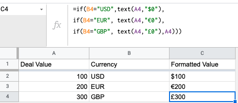
Let’s say our table looks like this: 

Deal Value	Currency	Formatted Value
100	USD
200	EUR
300	GBP

Let’s set on the third column the formula:

=IF(B2="USD",TEXT(A2,"$0"),
IF(B2="EUR", TEXT(A2,"€0"),
IF(B2="GBP", TEXT(A2,"£0"),A2)))

This will end up with this result:

In the formula above we are using two types of functions:

• IF: if the cell on the 2nd column has a value of “USD”, then:
• TEXT: format the text with the value of the 1st column, with this structure: the $ symbol and then the number with no numbers after the decimal point.

If we wanted to show the price with two numbers after the decimal point, the inner TEXT formula would be: TEXT(A2,”$0.00″).

This method is easy and simple but its downside is that we need to create an extra column for the formatted result. With a script, we can avoid that and format our existing values.

Change the Number Format to Currency with a Script

With the script, we can do pretty much the same thing as above, but now with formatting the existing value column. In our script, we will use the method setNumberFormat() where we set the correct currency symbol to the deal value. Let’s see the code:

function formatCurrencies() {
  let ss = SpreadsheetApp.getActiveSpreadsheet().getActiveSheet()
  let deal_values = ss.getRange("A2:A4").getValues().flat();
  const value_column = 1;
  const currency_column = 2;

  const currency_symbols = {
  'USD' : '$',
  'EUR' : '€',
  'GBP' : '£',
  'CAD' : '$',
  'ILS' : '₪',
  'AUD' : '$',
  'SGD' : '$',
  'JPY' : '¥'
  }

  for (i=0; i< deal_values.length; i++){
    var currency_name = ss.getRange(i+2,currency_column).getValue();
    var currency_symbol = currency_symbols[currency_name];
    ss.getRange(i+2,value_column).setNumberFormat(currency_symbol+"0")
  };
};

Here, we created the currency_symbols object with all the relevant acronyms as keys and the symbols as values.

Next, we iterate over the sheet rows, getting the currency name (i.e. USD), and getting the symbol from the object by the value ($).

Lastly, we set the formatting with setNumberFormat() with the symbol we found and the number (“0” means just the number without added numbers after the decimal point).

If we wanted to format the number with extra digits after the decimal point, we could write setNumberFormat(currency_symbol+”0.00″).